Serial Killings – Powerlaw or not?

Try to reproduce the analysis in Cosma Shalizi’s blogpost with scipy.

First, import things

from __future__ import absolute_import, print_function, division

import numpy as np
import pandas as pd
from scipy import stats
from statsmodels.distributions.empirical_distribution import ECDF
import matplotlib.pyplot as plt

from km3pipe.stats import bootstrap_fit
import km3pipe.style.moritz    # noqa

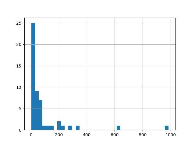
The data (times of killings) are in a text file, let’s write a small function to read them. We are interested in the time differences between the murders.

def get_time_deltas(fname):
    with open(fname) as f:
        raw_dates = f.read().split('\n')
    murder_dates = pd.Series(pd.to_datetime(raw_dates), name='Date')
    day = np.timedelta64(1, 'D')
    diffs = np.array(murder_dates.diff().iloc[1:-1]) / day
    diffs = pd.Series(diffs)
    return diffs


DATES_FILE = '../data/murder_dates.txt'
diffs = get_time_deltas(DATES_FILE)

diffs.hist(bins='auto')

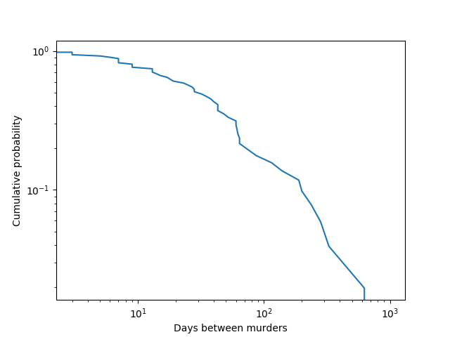
ecdf = ECDF(diffs)
days, eucdf = ecdf.x, 1 - ecdf.y
plt.loglog(days, eucdf)
plt.xlabel('Days between murders')
plt.ylabel('Cumulative probability')

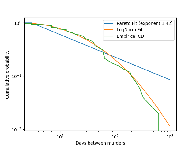
Let’s fit a powerlaw

pareto_idx, pareto_loc, pareto_scale = stats.pareto.fit(diffs)
pareto = stats.pareto(pareto_idx, pareto_loc, pareto_scale)

_ = bootstrap_fit(stats.pareto, diffs, n_iter=100)

Out:

--------------
pareto
--------------
  loc: +0.454 ∈ [+0.498, +0.498] (95%)
scale: -1.454 ∈ [-0.002, -0.002] (95%)
    b: +4.514 ∈ [+3.112, +3.112] (95%)

And a lognormal, because Gauss is not mocked.

lognorm_sig, lognorm_shape, lognorm_scale = stats.lognorm.fit(diffs)
lognorm = stats.lognorm(lognorm_sig, lognorm_shape, lognorm_scale)

_ = bootstrap_fit(stats.lognorm, diffs, n_iter=100)

Out:

--------------
lognorm
--------------
  loc: +2.176 ∈ [+6.613, +6.613] (95%)
scale: +2.363 ∈ [+3.000, +3.000] (95%)
    s: +23.764 ∈ [+35.268, +35.268] (95%)

plt.loglog(
    days,
    1 - pareto.cdf(days),
    label='Pareto Fit (exponent {:.3})'.format(pareto_idx + 1)
)
plt.loglog(days, 1 - lognorm.cdf(days), label='LogNorm Fit')
plt.loglog(days, eucdf, label='Empirical CDF')
plt.xlabel('Days between murders')
plt.ylabel('Cumulative probability')
plt.legend()

Total running time of the script: ( 0 minutes 18.279 seconds)