Histograms

Load a histogram from a file, plot it, draw random samples.

from __future__ import absolute_import, print_function, division

# Author: Moritz Lotze <mlotze@km3net.de>
# License: BSD-3

import h5py
import matplotlib.pyplot as plt
import numpy as np
import scipy.stats
import seaborn as sns

import km3pipe.style.moritz    # noqa

Out:

Loading style definitions from '/home/docs/checkouts/readthedocs.org/user_builds/km3pipe/conda/stable/lib/python3.5/site-packages/km3pipe/kp-data/stylelib/moritz.mplstyle'

Load the histogram from a file. a histogram is just bincounts + binlimits.

filename = "../data/hist_example.h5"

with h5py.File(filename, 'r') as f:
    counts = f['/hist/counts'][:]
    binlims = f['/hist/binlims'][:]

print(counts)
print(counts.shape)
print(binlims)
print(binlims.shape)

Out:

[  5  19  40  78  77  51  27  35  82 146 190 142  77  22   9]
(15,)
[11.82382487 12.60194812 13.38007137 14.15819462 14.93631788 15.71444113
 16.49256438 17.27068763 18.04881088 18.82693413 19.60505738 20.38318064
 21.16130389 21.93942714 22.71755039 23.49567364]
(16,)

create a distribution object

hist = scipy.stats.rv_histogram((counts, binlims))

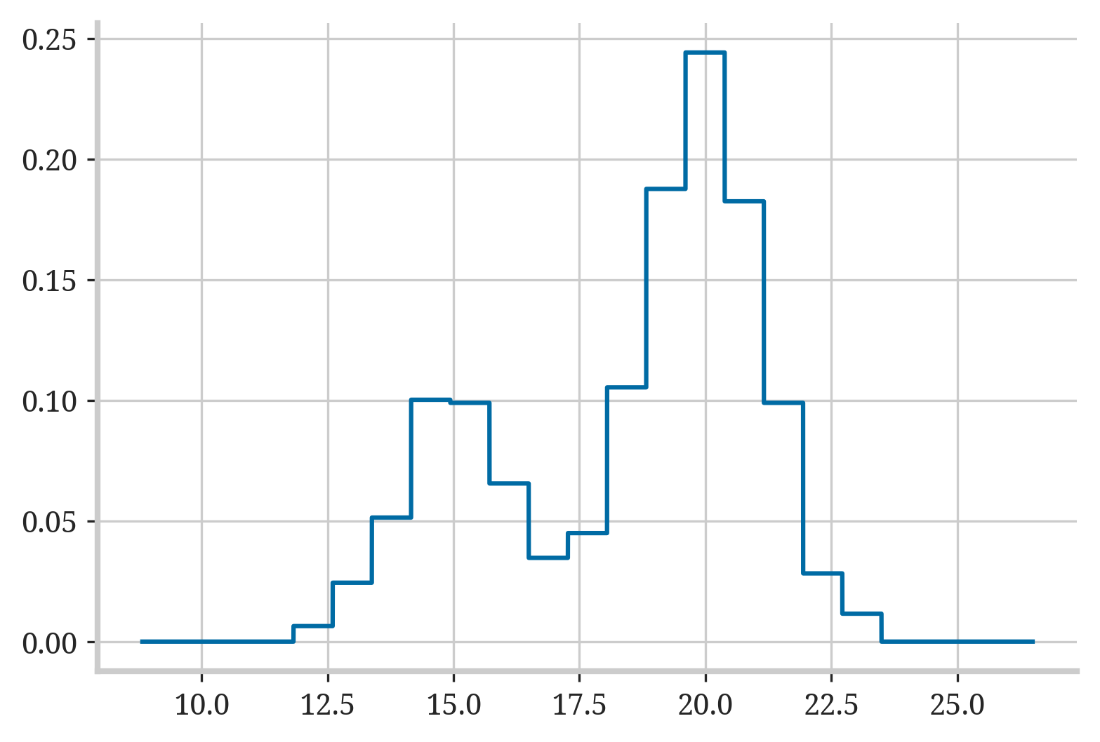
plot it

# make an x axis for plotting
padding = 3
n_points = 10000
x = np.linspace(binlims[0] - padding, binlims[-1] + padding, n_points)

plt.plot(x, hist.pdf(x))

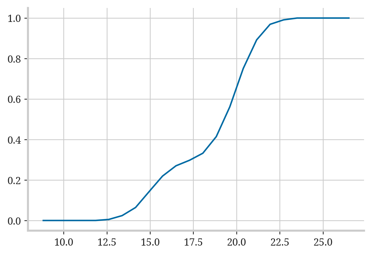
plot the cumulative histogram

plt.plot(x, hist.cdf(x))

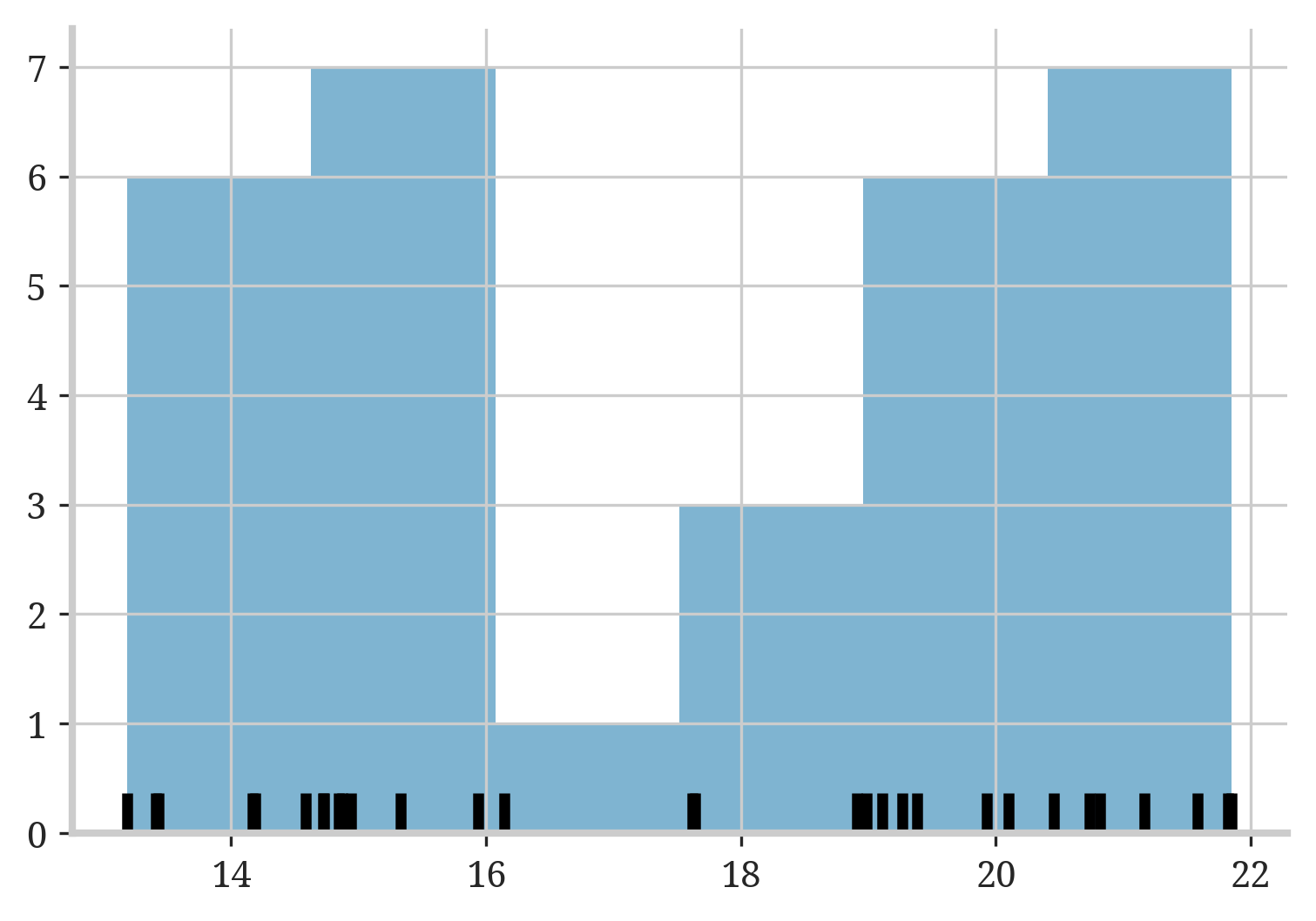
sample from the histogram (aka draw random variates)

n_sample = 30
sample = hist.rvs(size=n_sample)

let’s plot it (use seaborn to plot the data points as small vertical bars)

plt.hist(sample, bins='auto', alpha=.5)
sns.rugplot(sample, color='k', linewidth=3)

Total running time of the script: ( 0 minutes 0.211 seconds)