Fitting Distributions

Histograms, PDF fits, Kernel Density.

from __future__ import absolute_import, print_function, division

# Author: Moritz Lotze <mlotze@km3net.de>
# License: BSD-3

import matplotlib.pyplot as plt
import numpy as np
import statsmodels.api as sm

from scipy.stats import norm
from sklearn.mixture import GaussianMixture
from sklearn.model_selection import GridSearchCV
from sklearn.neighbors import KernelDensity

import km3pipe.style.moritz    # noqa

First generate some pseudodata: A bimodal gaussian, + noise.

N = 100
bmg = np.concatenate((
    np.random.normal(15, 1, int(0.3 * N)),
    np.random.normal(20, 1, int(0.7 * N))
))
noise_bmg = 0.5
data = np.random.normal(bmg, noise_bmg)[:, np.newaxis]

# make X axis for plots
x = np.linspace(5, 35, 3 * N + 1)

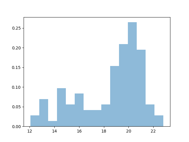
Histograms (nonparametric)

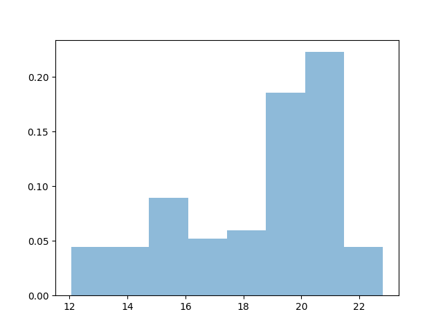
The simplest nonparametric density estimation tool is the Histogram. Choosing the binning manually can be tedious, however:

15 bins, spaced from data.min() to data.max().

plt.hist(data, bins=15, alpha=.5, normed=True)

Auto Binning (recommended)

Use builtin (numpy’s) heuristics to figure out best binning.

plt.hist(data, bins='auto', alpha=.5, normed=True)

Bayesian Blocks

TODO: Compute optimal segmentation of data with Scargle’s Bayesian Blocks. Produces bins of uneven width.

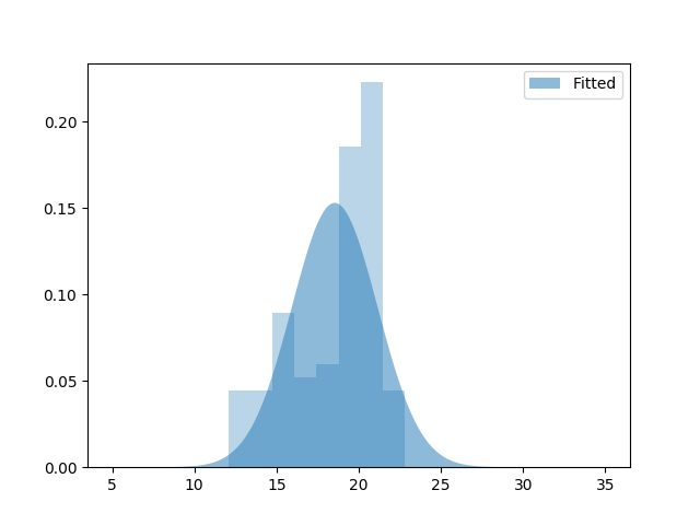
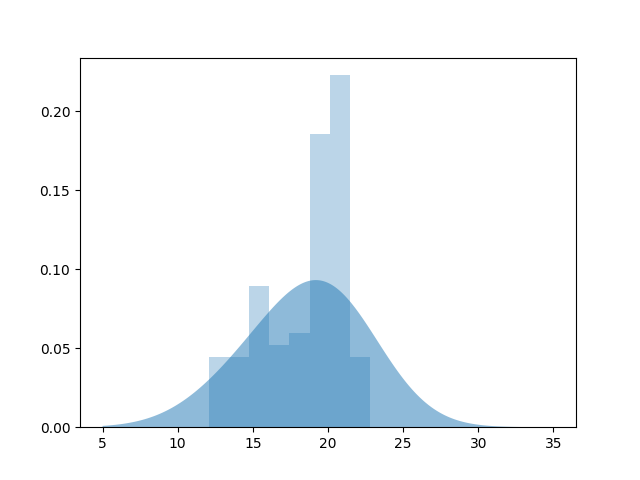
Fit Distribution via Maximum Likelihood

If we have a hypothesis what the distribution looks like (e.g. gaussian), and want to fit its parameters.

The nice thing is, you can define your own PDFs in scipy and fit it. Or take one from the dozens of pre-defined ones.

However, there is no bimodal gaussian implemented in scipy yet :/ In this case, either define it yourself, or use a GMM (below)

mu, sig = norm.fit(data)

plt.fill_between(x, norm(mu, sig).pdf(x), alpha=.5, label='Fitted')
plt.legend()
print('Unimodal Gaussian Fit:  Mean {:.4}, stdev {:.4}'.format(mu, sig))
plt.hist(data, bins='auto', alpha=.3, normed=True)

Out:

Unimodal Gaussian Fit:  Mean 18.54, stdev 2.608

As expected, the result is rather silly, since we are only fitting one of the two gaussians.

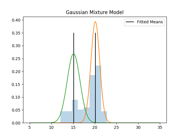
Fit Gaussian Mixture Model (GMM)

Assuming the data is the sum of one or more gaussians. Easily handles multidimensional case as well.

gmm = GaussianMixture(n_components=2, covariance_type='spherical')
gmm.fit(data)

mu1 = gmm.means_[0, 0]
mu2 = gmm.means_[1, 0]
var1, var2 = gmm.covariances_
wgt1, wgt2 = gmm.weights_
print(
    '''Fit:
      1: Mean {:.4}, var {:.4}, weight {:.4}
      2: Mean {:.4}, var {:.4}, weight {:.4}
'''.format(mu1, var1, wgt1, mu2, var2, wgt2)
)

plt.hist(data, bins='auto', alpha=.3, normed=True)
plt.vlines((mu1, mu2), ymin=0, ymax=0.35, label='Fitted Means')
plt.plot(x, norm.pdf(x, mu1, np.sqrt(var1)))
plt.plot(x, norm.pdf(x, mu2, np.sqrt(var2)))
plt.legend()
plt.title('Gaussian Mixture Model')

Out:

Fit:
      1: Mean 20.12, var 1.028, weight 0.685
      2: Mean 15.11, var 2.205, weight 0.315

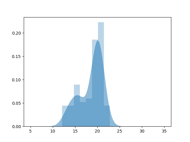
Kernel Density: (non-parametric)

If we have no strong assumptions about the underlying pdf.

“Smooth out” each event with a kernel (e.g. gaussian) of a certain bandwidth, then add together all these mini-functions.

The “bandwidth” (width of the kernel function) depends on the data, and can be estimated using cross-validation + maximum likelihood

in Statsmodels

dens = sm.nonparametric.KDEUnivariate(data)
dens.fit()

kde_sm = dens.evaluate(x)
plt.fill_between(x, kde_sm, alpha=.5, label='KDE')
plt.hist(data, bins='auto', alpha=.3, normed=True)

in scikit-learn

params = {'bandwidth': np.logspace(-2, 2, 50)}
grid = GridSearchCV(KernelDensity(), params)
grid.fit(data)

print("best bandwidth: {0}".format(grid.best_estimator_.bandwidth))

# use the best estimator to compute the kernel density estimate
kde_best = grid.best_estimator_
kde_sk = np.exp(kde_best.score_samples(x[:, np.newaxis]))
plt.fill_between(x, kde_sk, alpha=.5, label='KDE')
plt.hist(data, bins='auto', alpha=.3, normed=True)

Out:

best bandwidth: 3.3932217718953264

References

• B.W. Silverman, “Density Estimation for Statistics and Data Analysis”
• Hastie, Tibshirani and Friedman, “The Elements of Statistical Learning: Data Mining, Inference, and Prediction”, Springer (2009)
• Liu, R., Yang, L. “Kernel estimation of multivariate cumulative distribution function.” Journal of Nonparametric Statistics (2008)

Total running time of the script: ( 0 minutes 3.621 seconds)