Basic Analysis Example

from __future__ import absolute_import, print_function, division

# Authors: Tamás Gál <tgal@km3net.de>, Moritz Lotze <mlotze@km3net.de>
# License: BSD-3
# Date: 2017-10-10
# Status: Under construction...

Preparation

The very first thing we do is importing our libraries and setting up the Jupyter Notebook environment.

import matplotlib.pyplot as plt    # our plotting module
import pandas as pd    # the main HDF5 reader
import numpy as np    # must have
import km3pipe as kp    # some KM3NeT related helper functions
import seaborn as sns    # beautiful statistical plots!

this is just to make our plots a bit “nicer”, you can skip it

import km3pipe.style
km3pipe.style.use("km3pipe")

Out:

Loading style definitions from '/home/docs/checkouts/readthedocs.org/user_builds/km3pipe/conda/stable/lib/python3.5/site-packages/km3pipe/kp-data/stylelib/km3pipe.mplstyle'

Accessing the Data File(s)

In the following, we will work with one random simulation file with reconstruction information from JGandalf which has been converted from ROOT to HDF5 using the tohdf5 command line tool provided by KM3Pipe.

You can find the documentation here: https://km3py.pages.km3net.de/km3pipe/cmd.html#tohdf

Note for Lyon Users

If you are working on the Lyon cluster, you can activate the latest KM3Pipe with the following command (put it in your ~/.bashrc to load it automatically in each shell session):

source $KM3NET_THRONG_DIR/src/python/pyenv.sh

Converting from ROOT to HDF5 (if needed)

Choose a file (take e.g. one from /in2p3/km3net/mc/…), load the appropriate Jpp/Aanet version and convert it via:

tohdf5 --aa-format=the_file.root --ignore-hits --skip-header

Note that you may have to --skip-header otherwise you might encounter some segfaults. There is currently a big mess of different versions of libraries in several levels of the MC file processings.

The --ignore-hits will skip the hit information, so the converted file is much smaller (normally around 2-3 MBytes). Skip this option if you want to read the hit information too. The file will still be smaller than the ROOT file (about 1/3).

Luckily, a handful people are preparing the HDF5 conversion, so in future you can download them directly, without thinking about which Jpp or Aanet version you need to open them.

First Look at the Data

filepath = "data/basic_analysis_sample.h5"

We can have a quick look at the file with the ptdump command in the terminal:

ptdump filename.h5

For further information, check out the documentation of the KM3NeT HDF5 format definition: http://km3pipe.readthedocs.io/en/latest/hdf5.html

The /event_info table contains general information about each event. The data is a simple 2D table and each event is represented by a single row.

Let’s have a look at the first few rows:

event_info = pd.read_hdf(filepath, '/event_info')
print(event_info.head(5))

Out:

det_id  frame_index  livetime_sec  ...  weight_w3  run_id  event_id
0      -1            5             0  ...    0.07448       1         0
1      -1            8             0  ...    0.13710       1         1
2      -1           13             0  ...    0.11890       1         2
3      -1           15             0  ...    0.29150       1         3
4      -1           18             0  ...    0.10220       1         4

[5 rows x 17 columns]

Next, we will read out the MC tracks which are stored under /mc_tracks.

tracks = pd.read_hdf(filepath, '/mc_tracks')

also read event info, for things like weights

info = pd.read_hdf(filepath, '/event_info')

It has a similar structure, but now you can have multiple rows which belong to an event. The event_id column holds the ID of the corresponding event.

print(tracks.head(10))

Out:

bjorkeny     dir_x     dir_y     dir_z  ...   pos_z  time  type  event_id
0  0.057346 -0.616448 -0.781017 -0.100017  ... -71.802     0   -14         0
1  0.000000  0.488756 -0.535017 -0.689111  ... -71.802     0    22         0
2  0.000000 -0.656758 -0.746625 -0.105925  ... -71.802     0   -13         0
3  0.000000  0.412029 -0.878991 -0.240015  ... -71.802     0  2112         0
4  0.000000 -0.664951 -0.468928  0.581332  ... -71.802     0  -211         0
5  0.437484  0.113983  0.914457  0.388298  ...  30.360     0   -14         1
6  0.000000 -0.345462  0.923065 -0.169138  ...  30.360     0    22         1
7  0.000000  0.381285  0.828365  0.410406  ...  30.360     0   -13         1
8  0.000000 -0.191181  0.907296  0.374518  ...  30.360     0  3122         1
9  0.000000 -0.244006  0.922082  0.300377  ...  30.360     0   321         1

[10 rows x 15 columns]

We now are accessing the first track for each event by grouping via event_id and calling the first() method of the Pandas.DataFrame object.

primaries = tracks.groupby('event_id').first()

Here are the first 5 primaries:

print(primaries.head(5))

Out:

bjorkeny     dir_x     dir_y     dir_z  ...    pos_y   pos_z  time  type
event_id                                          ...
0         0.057346 -0.616448 -0.781017 -0.100017  ...   67.589 -71.802     0   -14
1         0.437484  0.113983  0.914457  0.388298  ... -109.844  30.360     0   -14
2         0.549859 -0.186416 -0.385939 -0.903493  ...  101.459 -30.985     0    14
3         0.056390 -0.371672  0.550002 -0.747902  ...   15.056  24.474     0   -14
4         0.049141 -0.124809 -0.979083  0.160683  ...   88.981 -65.848     0    14

[5 rows x 14 columns]

Creating some Fancy Graphs

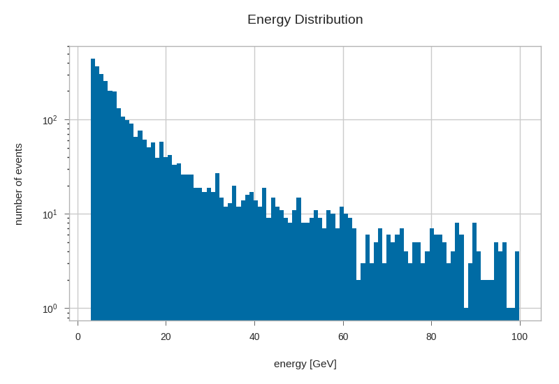
primaries.energy.hist(bins=100, log=True)
plt.xlabel('energy [GeV]')
plt.ylabel('number of events')
plt.title('Energy Distribution')

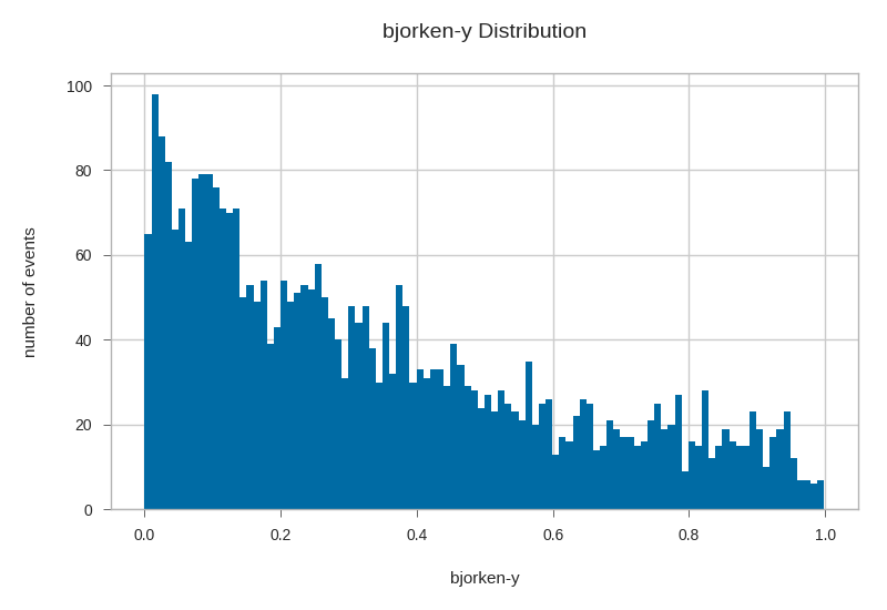
primaries.bjorkeny.hist(bins=100)
plt.xlabel('bjorken-y')
plt.ylabel('number of events')
plt.title('bjorken-y Distribution')

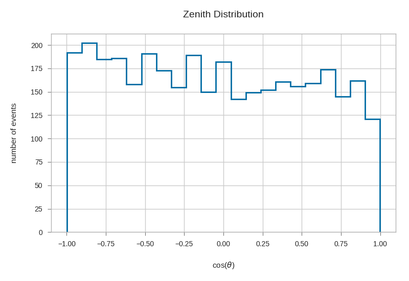
zeniths = kp.math.zenith(primaries.filter(regex='^dir_.?$'))
primaries['zenith'] = zeniths

plt.hist(np.cos(primaries.zenith), bins=21, histtype='step', linewidth=2)
plt.xlabel(r'cos($\theta$)')
plt.ylabel('number of events')
plt.title('Zenith Distribution')

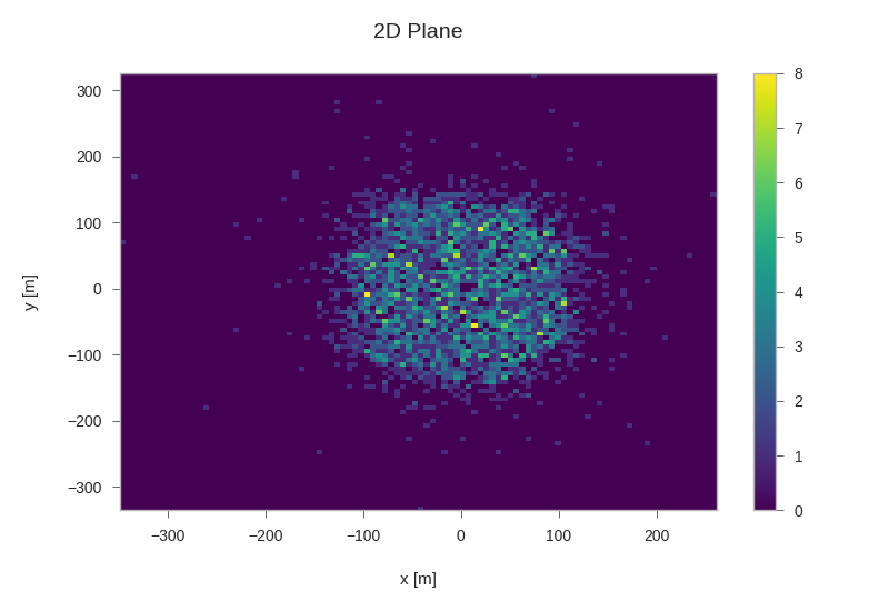
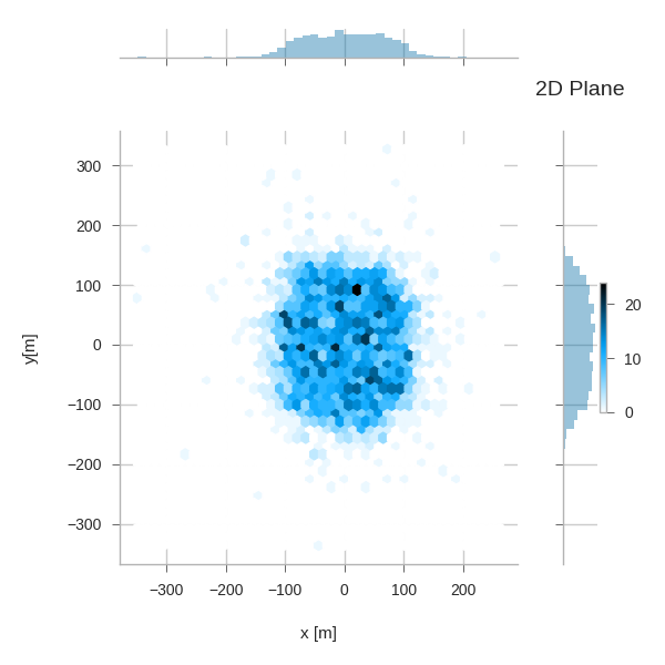
Starting positions of primaries

plt.hist2d(primaries.pos_x, primaries.pos_y, bins=100, cmap='viridis')
plt.xlabel('x [m]')
plt.ylabel('y [m]')
plt.title('2D Plane')
plt.colorbar()

If you have seaborn installed (pip install seaborn), you can easily create nice jointplots:

try:
    import seaborn as sns    # noqa
    km3pipe.style.use("km3pipe")    # reset matplotlib style
except:
    print("No seaborn found, skipping example.")
else:
    g = sns.jointplot('pos_x', 'pos_y', data=primaries, kind='hex')
    g.set_axis_labels("x [m]", "y[m]")
    plt.subplots_adjust(right=0.90)    # make room for the colorbar
    plt.title("2D Plane")
    plt.colorbar()
    plt.legend()

Out:

Loading style definitions from '/home/docs/checkouts/readthedocs.org/user_builds/km3pipe/conda/stable/lib/python3.5/site-packages/km3pipe/kp-data/stylelib/km3pipe.mplstyle'

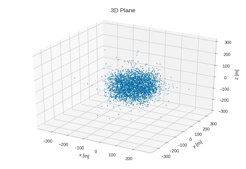
from mpl_toolkits.mplot3d import Axes3D    # noqa
fig = plt.figure()
ax = fig.add_subplot(111, projection='3d')
ax.scatter3D(primaries.pos_x, primaries.pos_y, primaries.pos_z, s=3)
ax.set_xlabel('x [m]', labelpad=10)
ax.set_ylabel('y [m]', labelpad=10)
ax.set_zlabel('z [m]', labelpad=10)
ax.set_title('3D Plane')

gandalfs = pd.read_hdf(filepath, '/reco/gandalf')
print(gandalfs.head(5))

Out:

beta0     beta1        chi2  ...  type  upgoing_vs_downgoing  event_id
0  0.016788  0.011857  -53.119816  ...   0.0             -0.274836         0
1  0.007835  0.005533  -32.504874  ...   0.0              3.907941         1
2  0.012057  0.008456  -81.195134  ...   0.0             -0.385038         2
3  0.007858  0.005554 -200.985734  ...   0.0             -0.809872         3
4  0.011166  0.007366  -89.451264  ...   0.0             -0.167897         4

[5 rows x 83 columns]

gandalfs.columns

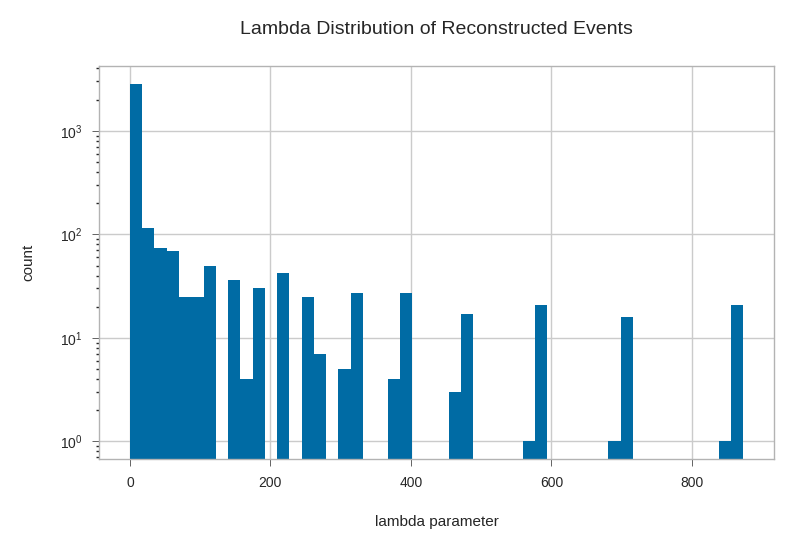
plt.hist(gandalfs['lambda'], bins=50, log=True)
plt.xlabel('lambda parameter')
plt.ylabel('count')
plt.title('Lambda Distribution of Reconstructed Events')

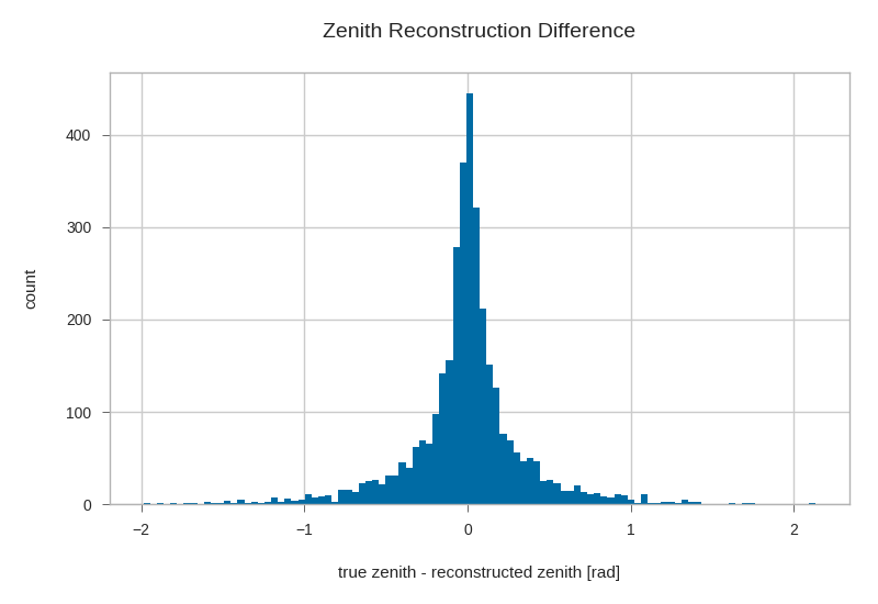
gandalfs['zenith'] = kp.math.zenith(gandalfs.filter(regex='^dir_.?$'))

plt.hist((gandalfs.zenith - primaries.zenith).dropna(), bins=100)
plt.xlabel(r'true zenith - reconstructed zenith [rad]')
plt.ylabel('count')
plt.title('Zenith Reconstruction Difference')

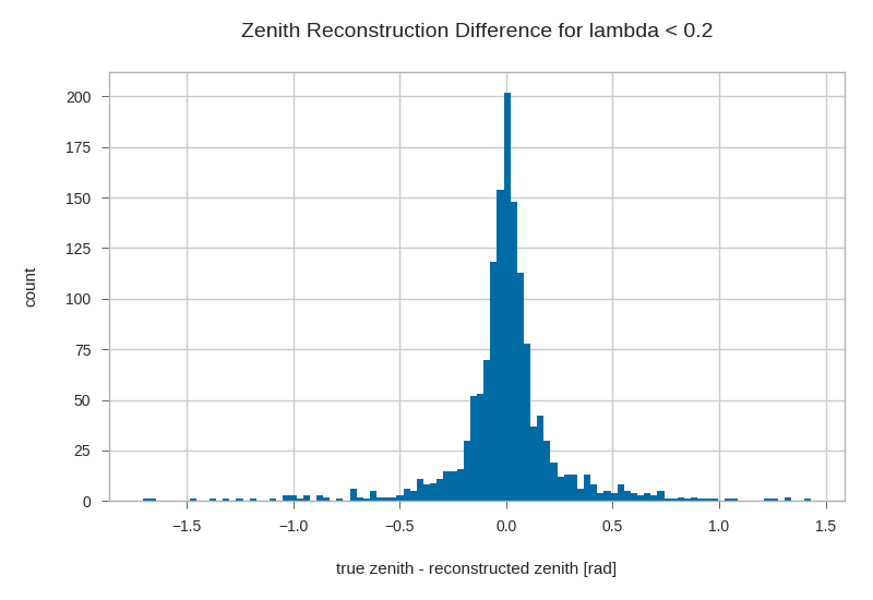
l = 0.2
lambda_cut = gandalfs['lambda'] < l
plt.hist((gandalfs.zenith - primaries.zenith)[lambda_cut].dropna(), bins=100)
plt.xlabel(r'true zenith - reconstructed zenith [rad]')
plt.ylabel('count')
plt.title('Zenith Reconstruction Difference for lambda < {}'.format(l))

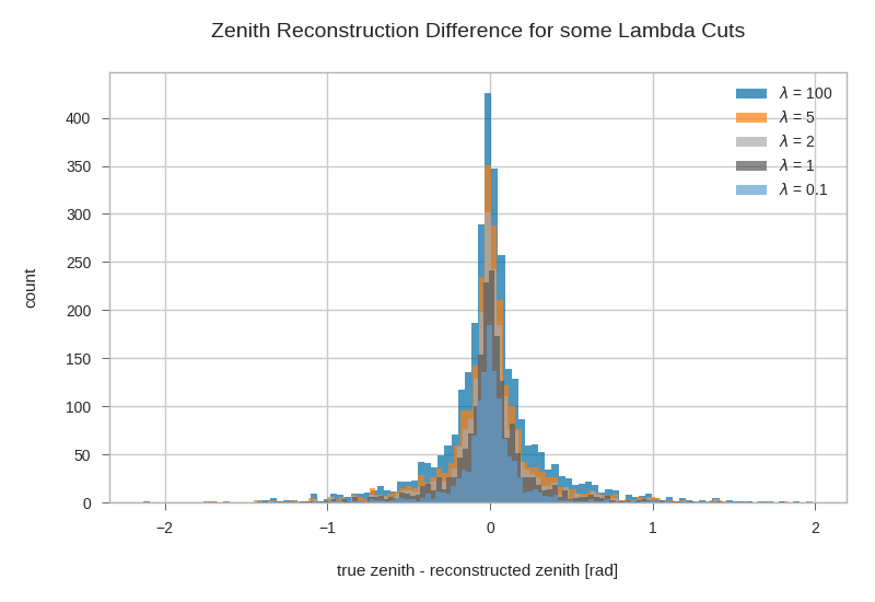
Combined zenith reco plot for different lambda cuts

fig, ax = plt.subplots()
for l in [100, 5, 2, 1, 0.1]:
    l_cut = gandalfs['lambda'] < l
    ax.hist((primaries.zenith - gandalfs.zenith)[l_cut].dropna(),
            bins=100,
            label=r"$\lambda$ = {}".format(l),
            alpha=.7)
plt.xlabel(r'true zenith - reconstructed zenith [rad]')
plt.ylabel('count')
plt.legend()
plt.title('Zenith Reconstruction Difference for some Lambda Cuts')

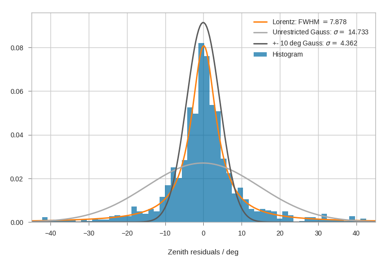
Fitting Angular resolutions

Let’s fit some distributions: gaussian + lorentz (aka norm + cauchy)

Fitting the gaussian to the whole range is a very bad fit, so we make a second gaussian fit only to +- 10 degree. Conversely, the Cauchy (lorentz) distribution is a near perfect fit (note that 2 gamma = FWHM).

from scipy.stats import cauchy, norm    # noqa

residuals = gandalfs.zenith - primaries.zenith
cut = (gandalfs['lambda'] < l) & (np.abs(residuals) < 2 * np.pi)
residuals = residuals[cut]
info[cut]

# convert rad -> deg
residuals = residuals * 180 / np.pi

pi = 180
# x axis for plotting
x = np.linspace(-pi, pi, 1000)

c_loc, c_gamma = cauchy.fit(residuals)
fwhm = 2 * c_gamma

g_mu_bad, g_sigma_bad = norm.fit(residuals)
g_mu, g_sigma = norm.fit(residuals[np.abs(residuals) < 10])

plt.hist(residuals, bins='auto', label='Histogram', normed=True, alpha=.7)
plt.plot(
    x,
    cauchy(c_loc, c_gamma).pdf(x),
    label='Lorentz: FWHM $=${:.3f}'.format(fwhm),
    linewidth=2
)
plt.plot(
    x,
    norm(g_mu_bad, g_sigma_bad).pdf(x),
    label='Unrestricted Gauss: $\sigma =$ {:.3f}'.format(g_sigma_bad),
    linewidth=2
)
plt.plot(
    x,
    norm(g_mu, g_sigma).pdf(x),
    label='+- 10 deg Gauss: $\sigma =$ {:.3f}'.format(g_sigma),
    linewidth=2
)
plt.xlim(-pi / 4, pi / 4)
plt.xlabel('Zenith residuals / deg')
plt.legend()

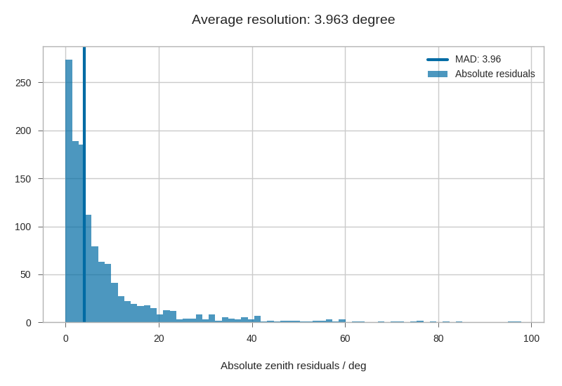
We can also look at the median resolution without doing any fits.

In textbooks, this metric is also called Median Absolute Deviation.

resid_median = np.median(residuals)
residuals_shifted_by_median = residuals - resid_median
absolute_deviation = np.abs(residuals_shifted_by_median)
resid_mad = np.median(absolute_deviation)

plt.hist(np.abs(residuals), alpha=.7, bins='auto', label='Absolute residuals')
plt.axvline(resid_mad, label='MAD: {:.2f}'.format(resid_mad), linewidth=3)
plt.title("Average resolution: {:.3f} degree".format(resid_mad))
plt.legend()
plt.xlabel('Absolute zenith residuals / deg')

Total running time of the script: ( 0 minutes 16.695 seconds)